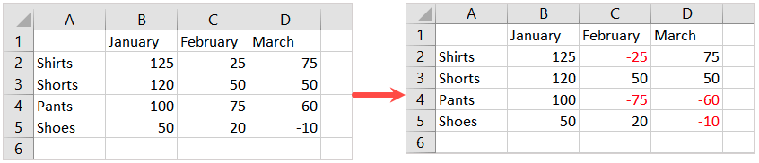
We’ll explain three methods for showing negative numbers as red in Excel. Use whichever you’re most comfortable with or works best for your sheet.
Format the Cells for Negative Red Numbers
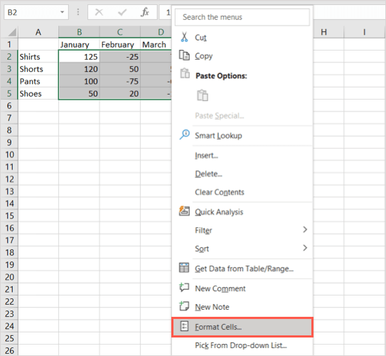
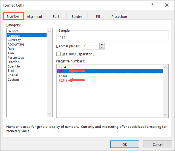
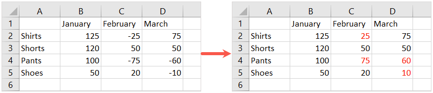
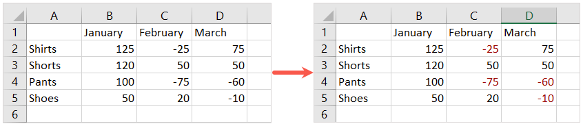
For the easiest way to format your negative numbers red, open your workbook to the spreadsheet and follow these steps. You should then see any negative numbers in your selected cells turn red while the positive numbers remain the same.
Create a Custom Format for Negative Red Numbers
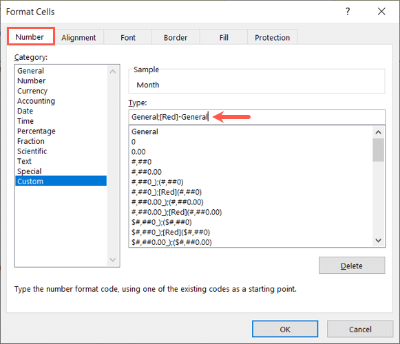
While the above is the simplest way to turn negative values red, you may not like the two choices you have. Perhaps you’d like to keep the negative sign (-) in front of the number. For this, you can create a custom number format. Now you’ll see your worksheet update and turn negative numbers red while retaining the minus signs in front of the numbers.
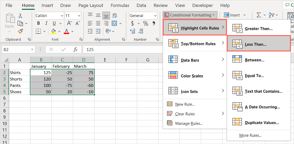
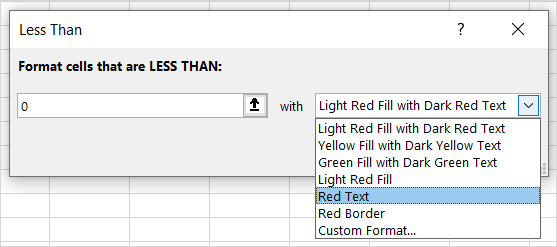
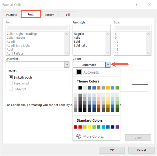
Use Conditional Formatting for Negative Red Numbers
Another option to make negative numbers red in Excel is with a conditional formatting rule. The advantage to this method is that you can choose the shade of red you want or apply additional formatting such as changing the cell color or making the font bold or underlined. You’ll then see your selected cells update to display negative numbers in a red font color and any other formatting you chose. With built-in ways to show negative numbers red in Excel, you can make sure those numbers stand out from the rest in your sheet. For more Excel tutorials, look at ways to convert text to numbers in your spreadsheet.